MATLAB Testing Tools
Overview
This tutorial explains the main features of OCUDU MATLAB, a MATLAB-based project for testing OCUDU. More specifically, this tutorial will show how to generate a new set of test vectors for the OCUDU tests, how to analyze the uplink IQ samples recorded by the OCUDU gNB, and how to run end-to-end, link-level simulations for testing PHY components of OCUDU. This will be done across three independent sections.
OCUDU MATLAB offers three main tools: the test vector generators, the uplink analyzers and the link-level simulators.
Test Vector Generation
Test vectors are mainly used to test, develop and debug the PHY components of OCUDU. This tutorial will show how to generate the set of vectors used for unit testing inside the OCUDU repository.
Signal Analyzers
The signal analyzers are useful for testing the uplink chain of the gNB. Specifically, they provide visual hints about the signal quality in the uplink slots.
Simulators
The simulators can be used to estimate the performance of the PHY uplink channels under different configurations and channel conditions provided by MATLAB’s 3GPP-compliant models.
Set-Up Considerations
For this application note, the following hardware and software are used:
- A PC with Ubuntu 24.04 LTS
- OCUDU MATLAB
- OCUDU
- MathWorks MATLAB (R2024b or R2025b) with the 5G Toolbox
Running the OCUDU MATLAB testing suite requires a working and licensed copy of MATLAB and its 5G Toolbox.
Installation
Assuming that OCUDU and MATLAB have both been downloaded and installed, the next step is to download OCUDU MATLAB.
This can be done with the following command:
git clone https://gitlab.com/ocudu/ocudu_elements/ocudu-matlab
This tutorial assumes that OCUDU is installed in the users home directory.
Once it has been downloaded, the working directory for OCUDU MATLAB should be added to MATLAB’s search path. This can be done from the MATLAB console with the following command:
cd ~/ocudu-matlab
addpath .
To verify you have added OCUDU MATLAB successfully to MATLAB’s search path, run the following command (again from the MATLAB console):
runtests('unitTests', Tag='matlab code')
If successful, the final section of the output should look similar to:
ans =

  1x131 TestResult array with properties:

    Name
    Passed
    Failed
    Incomplete
    Duration
    Details

Totals:
   131 Passed, 0 Failed, 0 Incomplete.
   242.2176 seconds testing time.
- Test Vectors
- Analyzers
- Simulators
The PHY components of OCUDU can be tested by feeding each component with vectors of input data and comparing the resulting output with their expected values. In this section of the tutorial we will learn how to generate these test vectors with OCUDU MATLAB and add the corresponding tests to the OCUDU main code.
Test vector generation
The files ocudu<ComponentName>Unittest.m in the main directory of OCUDU MATLAB provide the classes for
generating such PHY input–output test vectors. This is done by leveraging MATLAB 5G Toolbox. These classes inherit from
the MATLAB matlab.unittest.TestCase class, meaning all of the tools within MATLAB’s unit
testing framework can be used with them. To facilitate the generation of test vectors, a simplified interface
is provided with OCUDU MATLAB.
To generate the test vectors for all PHY components the following code needs to be run from the MATLAB console:
runOCUDUunittest('all', 'testvector')
This will generate a .h file, with the vector descriptions, and a .tar.gz file, with the actual test vectors, for each of the PHY components and place them in the folder ~/ocudu-matlab/testvector_outputs.
The test vectors for a single PHY component can also be generated. This is done by replacing all with the name of the desired
component, as per its declaration in ~/ocudu/include/ocudu/. For example, the test vectors for the channel estimator,
whose interface is declared in ~/ocudu/include/ocudu/phy/upper/signal_processors/port_channel_estimator.h, can be
generated with the following command:
runOCUDUunittest('port_channel_estimator', 'testvector')
Once the test vectors have been generated, the pairs of .h and tar.gz files in the testvector_outputs folder
should be transferred to the ocuduVectorTests folder with the MATLAB command:
ocuduTest.copyOCUDUtestvectors('testvector_outputs', 'ocuduVectorTests')
By default, executing runOCUDUunittest will always generate the same test vectors. To generate a random set of vectors,
we simply add the RandomShuffle option:
runOCUDUunittest('all', 'testvector', RandomShuffle=true)
Build and run the vector tests
The folder ocuduVectorTests contains C++ code that, together with the test vectors generated above, can be imported into OCUDU as a plugin:
cd ~/ocudu
mkdir plugins
cd plugins
ln -s ~/ocudu-matlab/ocuduVectorTests ocudu_vectortests
cd ..
Next, make sure that plugins are imported in OCUDU when building the project:
cmake -B buildplugins -DENABLE_PLUGINS:BOOL=ON
CMake will notify the inclusion of the vector tests with the message
-- Adding plugin: plugins/ocudu_vectortests
Finally, compile and run the tests with
cmake --build buildplugins -j $(nproc) --target all_vector_tests
ctest --test-dir buildplugins -j $(nproc) -L vectortest
OCUDU MATLAB provides some tools to analyze the signal received by the OCUDU gNB and help debugging the uplink channels. These
can be found in apps/analyzers. In this tutorial, we will focus on the analyzer for PUSCH transmissions; for the other
analyzers, which are very similar, please follow the instruction in their Help:
% The Resource Grid analyzers only plots the energy map of a slot.
>> help ocuduResourceGridAnalyzer

% For analyzing PUCCH transmissions.
>> help ocuduPUCCHAnalyzer

% For analyzing PRACH transmissions.
>> help ocuduPRACHAnalyzer

% For visualizing the allocated PHY channels.
>> help ocuduAllocationAnalyzer
To use the PUSCH analyzer, the gNB needs to be configured to collect IQ samples. This can be done with by adding the following snippet to the gNB configuration file:
log:
  filename: /tmp/gnb.log                         # save the log to a specified file
  phy_level: debug                               # debug log level for PHY layer set to debug
  phy_rx_symbols_filename: /tmp/iq.bin           # save IQ samples to a specified file
and running the gNB as usual:
sudo ./gnb -c config.yml
The generated IQ samples will occupy a large amount of disk space. It is recommended to not run the gNB with this configuration for too long.
After running the gNB, open the gnb.log and locate a PUSCH transmission to analyze. The following example shows the PUSCH transmission that will be
analyzed in this tutorial:
2026-03-08T19:14:54.738749 [Upper PHY] [I] [  690.17] RX_SYMBOL: sector=0 offset=79705 size=8568
2026-03-08T19:14:54.738854 [UL-PHY1 ] [D] [  690.17] PUSCH: rnti=0x4601 h_id=0 prb=[3, 6) symb=[0, 14) mod=QPSK rv=0 tbs=11 crc=OK iter=1.0 sinr=20.1dB t=182.0us uci_t=0.0us ret_t=0.0us
   rnti=0x4601
   h_id=0
   bwp=[0, 51)
   prb=[3, 6)
   symb=[0, 14)
   oack=0
   ocsi1=0
   part2=entries=[]
   alpha=0.0
   betas=[0, 0, 0]
   mod=QPSK
   tcr=0.1171875
   rv=0
   bg=2
   new_data=true
   n_id=1
   dmrs_mask={2, 7, 11}
   tbs_lbrm=3168bytes
   slot=690.17
   cp=normal
   nof_layers=1
   ports=0
   dc_position=306
   n_scr_id=1
   n_scid=false
   n_cdm_g_wd=2
   dmrs_type=1
   crc=OK
   iter=1.0
   max_iter=1
   min_iter=1
   nof_cb=1
   sinr_ch_est=26.9dB
   sinr_eq=23.9dB
   sinr_evm[sel]=20.1dB
   evm=0.06
   epre=+22.7dB
   rsrp=+22.7dB
   sinr_evm=20.1dB
   t_align=-0.2us
   cfo=-3.2Hz
Once the transmission has been located and selected, its description can be used to populate configuration options in the OCUDU MATLAB analyzer.
From the MATLAB console, run the following commands:
cd apps/analyzers
[carrier, pusch, extra] = ocuduParseLogs
You will then see the following output:
Copy the relevant section of the logs to the system clipboard (typically select and Ctrl+C), then switch back to MATLAB and press any key.
You should then copy the selected PUSCH transmission details from the log file, and paste it directly into the MATLAB console. The output should look like the following:
Parsing the following log section:

2026-03-08T19:14:54.738854 [UL-PHY1 ] [D] [  690.17] PUSCH: rnti=0x4601 h_id=0 prb=[3, 6) symb=[0, 14) mod=QPSK rv=0 tbs=11 crc=OK iter=1.0 sinr=20.1dB t=182.0us uci_t=0.0us ret_t=0.0us
   rnti=0x4601
   h_id=0
   bwp=[0, 51)
   prb=[3, 6)
   symb=[0, 14)
   oack=0
   ocsi1=0
   part2=entries=[]
   alpha=0.0
   betas=[0, 0, 0]
   mod=QPSK
   tcr=0.1171875
   rv=0
   bg=2
   new_data=true
   n_id=1
   dmrs_mask={2, 7, 11}
   tbs_lbrm=3168bytes
   slot=690.17
   cp=normal
   nof_layers=1
   ports=0
   dc_position=306
   n_scr_id=1
   n_scid=false
   n_cdm_g_wd=2
   dmrs_type=1
   crc=OK
   iter=1.0
   max_iter=1
   min_iter=1
   nof_cb=1
   sinr_ch_est=26.9dB
   sinr_eq=23.9dB
   sinr_evm[sel]=20.1dB
   evm=0.06
   epre=+22.7dB
   rsrp=+22.7dB
   sinr_evm=20.1dB
   t_align=-0.2us
   cfo=-3.2Hz
The function will ask for confirmation and for the sub-carrier spacing and the number of RBs in the resource grid:
Do you want to continue? [Y]/N y
Subcarrier spacing in kHz: 30
Grid size as a number of RBs: 51
Finally, ocuduParseLogs returns an nrCarrierConfig object, carrier, an nrPUSCHConfig object, pusch, and the extra structure with
additional information about the PUSCH transport block. It should look like the following:
carrier =

  nrCarrierConfig with properties:

              NCellID: 1
    SubcarrierSpacing: 30
         CyclicPrefix: 'normal'
            NSizeGrid: 51
           NStartGrid: 0
                NSlot: 17
               NFrame: 690

   Read-only properties:
       SymbolsPerSlot: 14
     SlotsPerSubframe: 2
        SlotsPerFrame: 20

pusch =

  nrPUSCHConfig with properties:

              NSizeBWP: 51
             NStartBWP: 0
            Modulation: 'QPSK'
             NumLayers: 1
           MappingType: 'A'
      SymbolAllocation: [0 14]
                PRBSet: [3 4 5]
    TransformPrecoding: 0
    TransmissionScheme: 'nonCodebook'
       NumAntennaPorts: 1
                  TPMI: 0
      FrequencyHopping: 'neither'
     SecondHopStartPRB: 1
         BetaOffsetACK: 20
        BetaOffsetCSI1: 6.2500
        BetaOffsetCSI2: 6.2500
            UCIScaling: 1
                   NID: 1
                  RNTI: 17921
                NRAPID: []
                  DMRS: [1x1 nrPUSCHDMRSConfig]
            EnablePTRS: 0
                  PTRS: [1x1 nrPUSCHPTRSConfig]

extra =

  struct with fields:

                      RV: 0
          TargetCodeRate: 0.1172
    TransportBlockLength: 88
              dcPosition: 306
The final step is to run the PUSCH analyzer, providing as inputs the objects just created by ocuduParseLogs,
the path to the IQ record, the offset and the length of the slot (both expressed as a number of IQ samples).
Both the offset and the length of the slot can be found in the log file, on a line like the following one
2026-03-08T19:14:54.738749 [Upper PHY] [I] [ 690.17] RX_SYMBOL: sector=0 offset=79705 size=8568
The slot ID ([ 690.17] in our example) should be the same as that of the PUSCH log.
The command to run the PUSCH analyzer from the MATLAB console is:
ocuduPUSCHAnalyzer(carrier, pusch, extra, '/tmp/iq.bin', 79705, 8568)
The block CRC is OK.
This should then output figures displaying the slot energy distribution, the magnitude of the estimated channel, the phase of the estimated channel, the equalized constellation and the received soft bit distribution.
The following figures show these:
| Slot Energy Distribution | Magnitude of the Estimated Channel | Phase of the Estimated Channel |
|---|---|---|
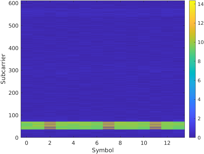 | 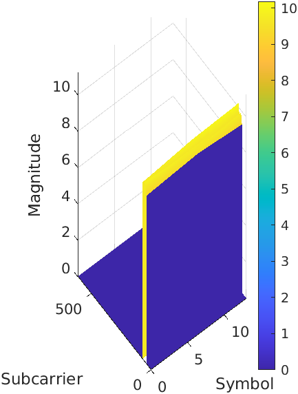 |  |
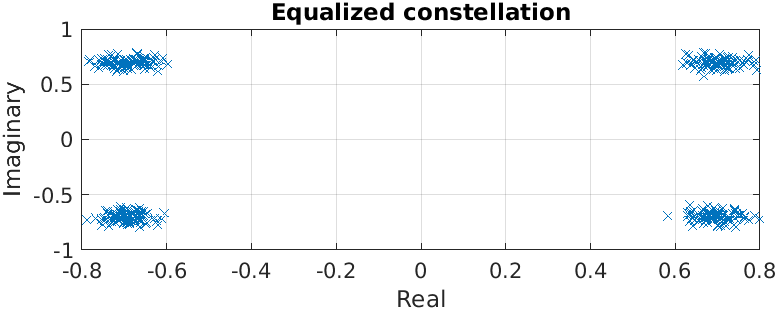 | 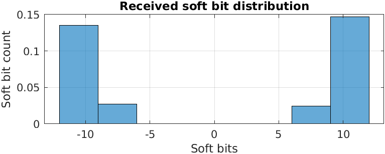 |
|---|
This example demonstrates how to test the throughput and BLER performance of the OCUDU gNB’s own PUSCH processor using OCUDU MATLAB simulators. By leveraging MATLAB’s 5G Toolbox we can build a simulation set-up that is as close as possible to the one required by 3GPP conformance tests (see TS38.104 and TS38.141). Although not fully representative of a real-world deployment with RUs and over-the-air transmission, these simulation are useful for obtaining a first estimation of the performance of the system.
A similar workflow applies to the other simulators provided by OCUDU MATLAB, namely PUCCHPERF and PRACHPERF to evaluate the performance of the PUCCH and PRACH receivers, respectively.
Compiling the MEXs
The inclusion of OCUDU PHY blocks into a MATLAB simulator is achieved by means of MEX functions, which are small C++ libraries that can be called from MATLAB. Therefore, the first step for running the OCUDU MATLAB simulators is to build the MEX executables.
First, we compile OCUDU with the ENABLE_EXPORT flag, to export (some of) its libraries for external
projects. This can be done from the command line with the following command:
cd ~/ocudu
cmake -B buildExport -DENABLE_EXPORT:BOOL=ON
cmake --build buildExport -j $(nproc)
This builds OCUDU inside buildExport and generates the file buildExport/ocudu.cmake, which
provides all the details required to import the necessary OCUDU CMake targets from external projects.
The ENABLE_EXPORT flag implies the generation of position-independent code (with the -fPIC compiler option) - as
a result, you may experience reduced performance when running the gNB.
The MEX libraries should now be built for OCUDU MATLAB. From the command line, run the following:
cd ~/ocudu-matlab/+ocuduMEX/source
cmake -B buildMEX -DOCUDU_BINARY_DIR:PATH="~/ocudu/buildExport" -DMatlab_ROOT_DIR:PATH="/path/to/MATLAB/R2024b"
cmake --build buildMEX -j $(nproc)
Finally, execute
cmake --install buildMEX
to copy the new MEX files into their final location, inside the class folders of +ocuduMEX/+phy.
To check that the above was run successfully, execute the following command from the main OCUDU MATLAB directory:
runtests('unitTests', Tag='mex code')
This should output the following, or similar, report:
ans =

  1x67 TestResult array with properties:

    Name
    Passed
    Failed
    Incomplete
    Duration
    Details

Totals:
   19 Passed, 0 Failed, 48 Incomplete.
   274.7124 seconds testing time.
You can then run:
runOCUDUunittest('all', 'testmex')
If successful, the runOCUDUunittest will generate test vectors, these will be fed into the MEX versions of OCUDU PHY components. An output similar to the following will be shown:
ans =
  1×1782 TestResult array with properties:

    Name
    Passed
    Failed
    Incomplete
    Duration
    Details
Totals:
   1404 Passed, 0 Failed, 378 Incomplete.
   41.8019 seconds testing time.
Running the PUSCH Simulator
The PUSCH simulator makes use of the class HARQEntity to manage parallel HARQ processes. The file implementing this class is distributed by MathWorks with the 5G Toolbox examples.
Licensed MATLAB users can obtain a copy by running
openExample('5g/Modeling5GNRTransportChannelsWithHARQExample')
at the command line. File HARQEntity.m must then be copied into the folder apps/simulators/PUSCHBLER/+matlablicense/ inside the OCUDU MATLAB project.
In the MATLAB console, from the main OCUDU MATLAB directory, a simulator object can be created as follows:
cd apps/simulators/PUSCHBLER
sim = PUSCHBLER
This should give the following output:
sim =

  PUSCHBLER with properties:

   Configuration
                         NCellID: 1
                            RNTI: 1
               SubcarrierSpacing: 15
                    CyclicPrefix: 'Normal'
                       NSizeGrid: 52
                          PRBSet: [0 1 2 3 4 5 6 7 8 9 10 11 12 13 14 15 16 17 18 19 20 21 22 23 24 25 26 27 28 29 30 31 32 … ] (1×52 double)
                SymbolAllocation: [0 14]
                     MappingType: 'A'
           DMRSConfigurationType: 1
                      DMRSLength: 1
          DMRSAdditionalPosition: 1
               DMRSTypeAPosition: 2
                        MCSTable: 'qam64'
                        MCSIndex: 0
              TransformPrecoding: false
                         NRxAnts: 1
                         NTxAnts: 1
                       NumLayers: 1
             FadingTimeEvolution: 'Slot independent'
                    DelayProfile: 'AWGN'
          CarrierFrequencyOffset: 0
         PerfectChannelEstimator: true
                      EnableHARQ: false
             ApplyOFHCompression: false
       MaximumLDPCIterationCount: 6
              ImplementationType: 'matlab'
                 QuickSimulation: true
    DisplaySimulationInformation: false
              DisplayDiagnostics: false
The simulation set-up can now be modified as desired by the user. In particular, the ImplementationType should be changed to ocudu. Doing
so allows the PHY components of OCUDU to be used (via the MEX libraries above) instead of those from the MATLAB 5G Toolbox.
This can be done with the following command:
sim.ImplementationType = 'ocudu'
A simulation can then be run to evaluate the throughput and BLER of the PUSCH transmission. This can be done by running sim([SNR Range], [# Frames]). An example simulation may look like the following:
sim(-8:-3, 10)
The resulting throughput and BLER estimations can then be plot with the following command:
sim.plot()
This will give the following output:
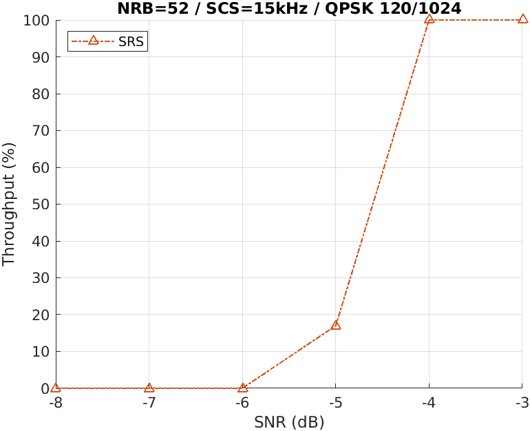 | 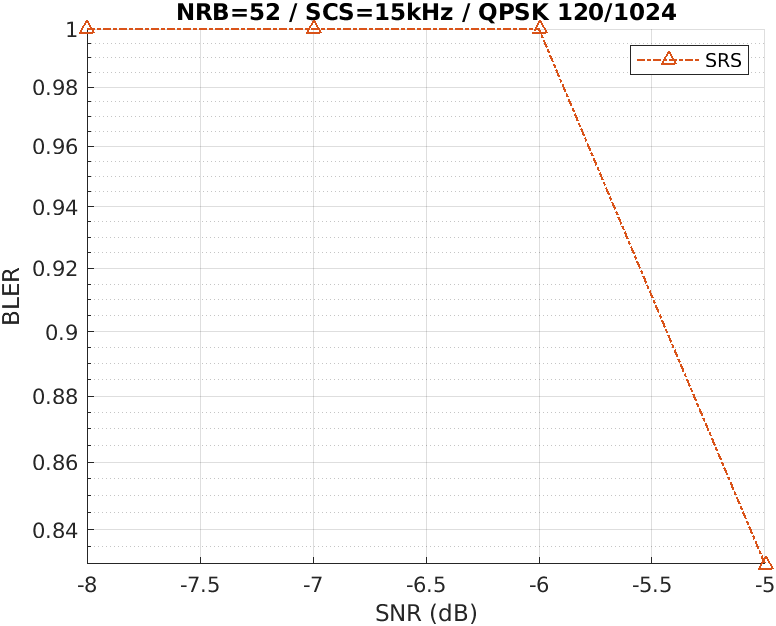 |
|---|